Credit Risk
Credit risk is the risk that a counterparty will fail to meet his payment obligation, resulting in a loss. This risk is historically considered the main risk for banks. Under BIS II a bank should asses its credit risk and retain capital for it.
In this section the methods available for assessing credit risk are explained. These are:
- Standardized approach<
- Internal Rating Based approach (IRB)
- Foundation
- Advanced
The main risk factors which need to be modelled in the Internal Rating Based approach (IRB) are the PD, LGD and EAD. How these factors work together to determine the credit risk is explained in the Internal Rating Based approach (IRB) chapter. How these factors can be modelled is discussed separately in the PD, LGD and EAD chapters.
Standardized approach
The standardized approach of BIS2 for credit risk is an elaboration of the BIS1 framework. The standardized approach allows additional segregation between risk, based on external risk ratings. For different types of claims different risk weights are given (for a particular risk grading). This section will give practical information on how to implement the standardized approach.
The idea behind the approach is to first categorise each claim and determine the credit exposure of the claim. Second determine the effect of eligible collateral from the claim. Third the risk of the counterparty is determined through external ratings. Fourth the external rating is mapped to a risk weight for the claim.
Categorise Claims
The standardised approach is calculated on the level of claims and not on the level of the counterparty. Each claim is assigned a risk weight, determining the capital necessary. Different rules apply to different type of claims. For this reason the portfolio will need to be divided into different types of claims. Make sure your entire portfolio is divided into one of the following categories. Claims on:
- Past due loans (this supersedes all other categories)
- Sovereigns
- Non-central government public sector entities (PSE’s)
- Multilateral development banks (MDB’s)
- Banks<
- Security firms
- Corporates<
- Retail counterparties
- Claims secured by residential property
- Claims part of the retail portfolio
- Claims secured by commercial real estate
- Higher risk categories (these supersede any other category except past due loans)
- Claims on sovereigns, PSE’s, banks and security firms rated below B-(S&P notation)
- Claims on corporates rated below BB- (S&P notation) (this supersedes the corporate category)
- Securitisation tranches rated between BB+ and BB-(S&P notation).
- Other items
- Gold bullion held in own vaults or on an allocated basis to the extent backed by bullion liabilities
- cash items in the process of collection.
- Remaining other
The more elaborate description of these claim types can be found in the BIS2 document page 19 through 27.
Off-balance sheet items should first be divided into the following categories:
- Commitments with an original majority up to one year. (20%)
- Commitments with an original majority over one year. (50%)
- Commitments which are unconditionally cancellable at any time by the bank without prior notice, or that effectively provide for automatic cancellation due to deterioration In a borrower’s credit worthiness. (0%)
- Direct credit substitutes, e.g. general guarantees of indebtedness (including standby letters of credit serving as financial guarantees for loans and securities) and acceptances (including endorsements with the character of acceptances). (100%)
- Sale and repurchase agreements and asset sales with recourse, where the credit
risk remains with the bank. (100%) - The lending of banks’ securities or the posting of securities as collateral by banks, including instances where these arise out of repo-style transactions (i.e. repurchase/reverse repurchase and securities lending/securities borrowing transactions). (100%)
- Forward asset purchases, forward deposits and partly-paid shares and
securities, which represent commitments with certain drawdown. (100%). - Transaction-related contingent items (e.g. performance bonds, bid bonds, warranties and standby letters of credit related to particular transactions). (50%)
- Note issuance facilities (NIFs) and revolving underwriting facilities (RUFs). (50%)
- short-term self-liquidating trade letters of credit arising from the movement of
goods (e.g. documentary credits collateralised by the underlying shipment), irrespective of the banks roll. (20%)
Dependant on the category, the off balance sheet item is transformed into a credit exposure equivalent. This is done by multiplying the value of the off balance sheet item with the appropriate credit conversion factor (CFF) which is given between brackets in the list above.
After the off balance sheet item has been categorised it can be allocated to one of the earlier mentioned claim types in order to determine the risk weight. The regulatory capital is calculated by multiplying the credit exposure equivalent by the risk weight.
Credit Risk Mitigation
The standardised approach allows for the incorporation of several types of credit risk mitigation in determining the regulatory capital for a claim. For a form of risk mitigation to qualify it should be legally enforceable. This means there should be a strong legal basis for actually obtaining the value of the risk mitigation, when necessary. The precise definition of legally enforceable is given in paragraph 117 and 118 of the BIS II paper.
As with the claims, the risk mitigation types are first categorised. Each category has its own rules for calculating the risk mitigation value. The following categories are identified:
- Collateral<
- On balance sheet netting
- Guarantees and credit derivatives<
- Miscellaneous
Collateral<
Different types of collateral may be incorporated in the capital calculations for the claim to which it is linked. This poses the problem of calculating the effect of the collateral. The standardised approach proposes two different methods for determining the impact of collateral. One of which is again split in two calculation methods:
In the simple approach the claim is split into the following parts.
- Collateralized part
- Collateralized by collateral type 1
- Collateralized by collateral type 2
- Etc…..
- Unsecured part
The type 1 and type 2 act as examples. A claim can be collateralized by many types of eligible collateral. For each part of the claim collateralized by different collateral the regulatory capital is separately calculated. For the collateralized part of the claim the regulatory capital is calculated by multiplying the value of the collateral by the risk weight assigned to that collateral item. The regulatory capital of the unsecured part of the claim is calculated by assigning the claim to one of the claim-categories and determining its grade.
In the comprehensive approach the value of both the claim and the collateral is adjusted. The claim is adjusted to represent possible claim growth. A claim could grow in exposure if for instance securities are lent. The collateral is adjusted to represent the collateral value loss due to market fluctuations. A separate adjustment is made to incorporate the risk of exchange rate changes when the collateral and the claim are in different currencies. After both values have been adjusted the latter is subtracted from the former leaving the exposure after collateral. The regulatory capital is calculated by multiplying the exposure after collateral by the risk weight of the claim. The haircuts for the claim and the collateral can either be calculated by the bank (in the Own Estimates of Haircuts approach) or the regulatory haircuts can be used (in the Standard Supervisory Haircuts approach).
On balance sheet netting
On balance sheet netting means that a debit exposure (a claim) is directly offset by a credit exposure. This is done with limited use of haircuts or further calculation. Regulatory capital will have to be calculated over the remaining (net) debit exposure if any. Basel states the following:
“Where a bank,
(a) has a well-founded legal basis for concluding that the netting or offsetting agreement is enforceable in each relevant jurisdiction regardless of whether the counterparty is insolvent or bankrupt;
(b) is able at any time to determine those assets and liabilities with the same counterparty that are subject to the netting agreement;
(c) monitors and controls its roll-off risks; and
(d) monitors and controls the relevant exposures on a net basis,
it may use the net exposure of loans and deposits as the basis for its capital adequacy calculation in accordance with the formula in paragraph 147. Assets (loans) are treated as exposure and liabilities (deposits) as collateral. The haircuts will be zero except when a currency mismatch exists. A 10-business day holding period will apply when daily mark-to market is conducted and all the requirements contained in paragraphs 151, 169, and 202 to 205 will apply.”
The formula referred to is the comprehensive approach for calculating regulatory capital. In essence the formula is used with claim and collateral haircuts of zero percent.
Guarantees and credit derivatives<
-Guarantees<
Guarantees given by the following institutions are eligible as risk mitigation:
- Sovereign entities, including BIS, IMF, European Central Bank, the European Community and multilateral development banks (a list of MDB’s is available in footnote 24 page 21 of the BIS2 paper)
- Public Sector Entities (PSE) (a decent definition of a Security firm is still required. Please post suggestions)
- Other entities rated A- or better. This includes parents, subsidiaries and affiliate companies.
A guarantee with a rating worse then the counterparty should be ignored (comments on the subject are appreciated, what is your opinion)
Furthermore there are several contractual and operational requirements which have to be met. Basically the contract has to be legally enforceable in any circumstance. There may be no exit clause freeing (reducing) the guarantor from his obligations.
If there is a materiality threshold before which the guarantor is not obliged to pay, this amount should be subtracted directly from the regulatory capital (it is unknown which capital should be used tier one, tier two or both).
If the guarantee does not cover all expected income (principle, interest, fees, etc.) but for instance only the principle, the uncovered income should be considered an unsecured claim. It is not clear how this should be accomplished; comments on the subject are welcome. A possibility would be to discount the expected interest payments and fees using the funding rate. The discounted value can then be added to the claim. If the guarantee is set in a different currency than the claim a currency haircut should be made on the guarantee amount.
The regulatory capital is calculated by using the guarantors risk weight for the guaranteed portion of the claim, and the counterparties risk weight for the unsecured portion of the claim.
In other words:
Ga = G * (1 – Hfx)
Ga = The guarantee amount after the currency mismatch haircut.
G = Value of the guarantee (contractually set)
Hfx = The appropriate currency mismatch haircut (Any insights in how to determine the appropriate haircut are welcome, please post comments on the subject)
RWA = (C + UI – Ga) * RWC + Ga * RWG
RWA = Risk Weighted Asset
C = Exposure of the claim
UI = Value of Unsecured Income (interest payments, fees, etc.)
RWC = Risk Weight of the Counterparty
RWG = Risk Weight of the Guarantor
RC = RWA * 8%
RC = Regulatory Capital<
- Credit Derivatives<
This section is still under construction. Comments, suggestions and articles are welcome.
Maturity Mismatch
This section is still under construction. Comments, suggestions and articles are welcome.
Other items relating to credit risk mitigation<
This section is still under construction. Comments, suggestions and articles are welcome.
Internal Rating Based approach (IRB)
The Internal Rating Based approach (IRB) allows banks to asses their credit risk using their own models. The approach is split into two possible methods, between which a bank must choose, Foundation and Advanced.
In this chapter the general logic behind the IRB approach is explained. This is followed by an explanation of the difference between the two methods (Foundation and Advanced). Finally the different types of assets for which the credit risk must be assessed are explained.
IRB basics
In this section the basic ideas behind the Internal Ratings Based approach are explained. First the concept of a credit loss distribution is explained. Secondly the method by which Basel calculates the expected and unexpected loss is explained.
Credit Loss Distribution
The goal of modelling credit risk is to determine the credit loss distribution. A credit loss is a loss due to debtors who fail to meet their payment obligations in one year. The distribution is a combination of probabilities and losses. For instance:
There is a probability of 2% for a credit loss of €50,000.- or less.
There is a probability of 7% for a credit loss of €100,000.- or less.
There is a probability of 16% for a credit loss of €150,000.- or less.
There is a probability of 31% for a credit loss of €200,000.- or less.
Etc.
These probabilities continue to grow until it is one. The probability of an endless credit loss or less is one. This is because all credit losses are endless or less.
If you have enough estimates of a probability for a loss of X or less a graph can be drawn. Such a graph is called a cumulative distribution function (CDF). The following example shows ten combinations of probabilities and credit loss. Each probability indicates the probability of the associated credit loss or less.
| Probability | Credit loss (or less) |
| 2% | € 50,000 |
| 7% | € 100,000 |
| 16% | € 150,000 |
| 31% | € 200,000 |
| 50% | € 250,000 |
| 69% | € 300,000 |
| 84% | € 350,000 |
| 93% | € 400,000 |
| 98% | € 450,000 |
| 99% | € 500,000 |
These probabilities and associated losses translate to the following CDF:
 |
The CDF graph shows the probability for each level of loss or less. This graph can be transformed into a distribution function by taking its derivative. This strips the “Cumulative” from the CDF. In our example the distribution function would look like this:
 |
The first graph shows the probability of a certain loss or less. The second graph shows the probability of a specific loss. A point on the first graph (the CDF) can be reconstructed from the second graph by adding all the probabilities equal to, or less than, the credit loss. In other words, a point on the first graph (the CDF) can be reconstructed from the loss distribution (the second graph) by taking the area under the graph up to and including the credit loss for which you wish to recreate the point.
The red area in the graph below represents the probability of €200,000 or less. The total value of this area is 31%, which is equal to the probability of €200,000 or less on the CDF graph.
 |
In these examples a normal distribution is used. The actual loss distribution can have any form.
Translating a loss distribution to capital
So why is this loss distribution so important? The purpose of holding capital is to ensure that a bank is capable of absorbing loss in an extreme situation. Basel defines an extreme situation as the point on the loss distribution with 99.9% probability of the associated credit loss or less. This is represented by the green and red area of the next graph.
 |
The green and red area combined make up 99.9% of the total area under the graph. In our example the point which represents the 99.9% probability is €559,025. This means there is a probability of 99.9% that the credit risk will be is €559,025 or less.
The green area in the graph represents 50% of the total area under the graph. In other words there is a 50% probability of this loss or less. This level of loss is called the expected loss. In our example the expected loss is €250,000. In other words there is a 50% probability for a loss of €250,000 or less. This part of the risk of loss should be covered by the provisions of a bank. This means that the banks provisions for credit risk should equal the expected loss.
The red area is the remainder between the expected loss and the loss at the 99.9% point. This remainder is called the unexpected loss. The regulatory capital is used to cover the unexpected loss. In our example we showed that the 99.9% point was at a loss of €559,025 and the expected loss was €250,000. Therefore the unexpected loss in our example is €559,025 - €250,000 = €309,025.
The sum of the provisions and the regulatory capital should equal the 99.9% loss. If for some reason the provisions are less than the expected loss, it should be compensated by holding extra regulatory capital.
In the next section we will discuss the method by which Basel attempts to model the credit loss distribution.
Vasicek model
The formula used to determine the regulatory capital is commonly referred to as the Vasicek model. The purpose of this model is to determine the expected loss (EL) and unexpected loss (UL) for a counterparty, as explained in the previous section. The first step in this model is to determine the expected loss. This is the average credit loss. There is a 50% change of realizing this loss or less. The expected loss is determined using three main ingredients:
PD: Probability of default, the average probability of default over a full economic cycle;
EAD: Exposure at default, the amount of money owed at the moment a counterparty goes into default;
LGD: Percentage of the EAD lost during a default.
The expected loss (EL) is equal to the PD times the LGD times the EAD:
EL = PD X LGD X EAD<
The expected loss is half the work of the model. The EL determines (roughly) the amount of provisions which should be taken (the essence of any provision is to save money for losses you expect in the future). The second half of the work is to determine the Unexpected Loss (UL). The UL is the additional loss in atypical circumstances, for which tier capital should be retained. The Vasicek model estimates the UL by determining the PD in a downturn situation. The model assumes that the EAD and LGD are not affected by dire circumstances. Both parameters are considered constant for a company. The model calculates the loss during a downturn situation (for instance an exceptionally bad economy) by multiplying the downturn PD times the LGD times the EAD. The UL is calculated by subtracting the expected loss from the loss during a downturn situation. In formula’s this equates to:
UL = (PDdownturn X LGD X EAD) – (PD X LGD X EAD),
which is equal to:
UL = (PDdownturn – PD) X LGD X EAD<
The PD in a downturn situation is determined using the average (through the cycle) PD. At this point Vasicek uses two different models. First it uses the Merton model. This model states that a counterparty defaults because it cannot meet its obligations at a fixed assessment horizon, because the value of its assets is lower than its due amount. Basically it states that the value of assets serve to pay off debt. The value of a company’s assets vary through time. If the asset value drops below the total debt, the company is considered in default. This logic allows credit risk to be modelled as a distribution of asset values with a certain cut-off point (called a default threshold), beyond which the company is in default. The area under the normal distribution of the asset value below the debt level of a company therefore represents the PD. The following figure shows a normal distribution of the assets values. The current asset value of this example is €1,000,000, the standard deviation is €200,000 and the total debt is €700,000. The probability of the asset value falling below €700,000 (the total debt level and therefore the default threshold) is equal to the area red area in the graph. As a company is considered in default if the asset value drops below the total debt, this probability is equal to the PD. In our Example the red area (PD) is 6.68%.
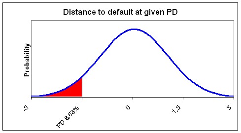 |
The logic used by Merton (shown in the graph above) can also be reversed. In Vasicek a PD (for instance calculated with a scorecard) is given as input. Instead of taking the default threshold (debt value) and inferring the PD as Merton does, Vasicek takes the PD and infers the default threshold. Vasicek does this using a standard normal distribution. This is a distribution with an average of zero and a standard deviation of one. This way the model measures how many standard deviations the current asset value is higher than the current debt level. In other words it measures the distance to default. The graph below shows that a PD of 6.68% means that the company is currently 1.5 standard deviations of its asset value away from default. By using the standard normal distribution the actual asset value, standard deviation and debt level becomes irrelevant. It is only necessary to know a PD and the distance to default can be determined.
Now that the PD has been transformed to a distance to default the second step of the model comes into play. In this step Vasicek uses the Gordy model. The distance to default is a through the cycle distance, because the PD used is through the cycle. In other words it is an average distance to default in an average situation. This distance to default (-1.5 in our example) will have to be transformed into a distance to default during an economic downturn. To do this a single factor model is used. It is assumed that the asset value of a company is correlated to a single factor. In other words, if the factor goes up the asset value goes up, if the factor goes down the asset value goes down. This factor is often referred to as the economy. This is done because it is intuitively logical that the asset value of a company is correlated to the economy. We will follow this tradition; however the factor is merely conceptual. It is assumed that there is a single common factor (whatever it may be) to which the asset value of all companies show some correlation. The common risk factor (the economy) is also assumed to be a standard normal distribution.
To recap we have a standard normal distribution representing the possible asset values, a default threshold inferred using the PD (-1.5 in our example), a standard normal distribution representing the economy to which the asset value is correlated and a correlation between the economy and the asset value. Using the correlation it is possible to determine the asset value distribution given a certain level of the economy. If the economy degrades the expected asset value will also decrease shifting the asset value distribution to the left. Furthermore the standard deviation will also decrease. In other words an asset value distribution given a certain level of the economy can be calculated using the correlation between the asset value and the economy. The following graphs give an example of how the asset value distribution can change as the economy level decreases.
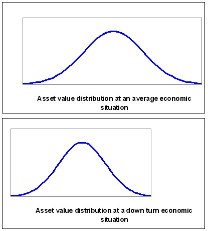 |
As the asset value distribution shifts the distance to default also shifts (decreases). The graphs below show the effect on the PD. The increase in the red area (and decrease in the distance to default) represents the increase in the PD due to adverse economic conditions.
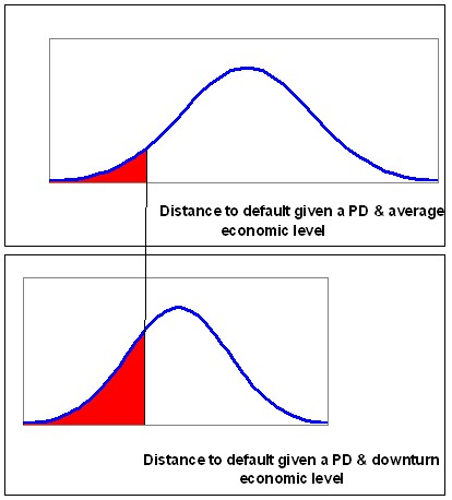 |
The degree in which the asset value distribution is deformed depends on the level of the economy which is assumed. The level of the economy is measured as the number of standard deviations the economy is from the average economy. For instance the economic level with a probability of 99.9% of occurring or better has a distance of 3.09 standard deviations from the average economy.
The new distance to default can be calculated by taking the average of the distance of the level of the economy (used to determine the downturn PD) and the distance to default, weighted by the correlation. In formula’s this equates to:
DistanceToDefaultDownturn = (1-r)^-0.5 X DistanceToDefault+ (r/(1-r))^0.5 X DistanceFromEconomy.
In our example the PD was 6.68% and the distance to default was -1.5. Now assume a counterparty has a 9% correlation to the economy. Secondly determine that the economic downturn level is the 99.9% worst possible economic level (used in BIS II). At this level the distance between the downturn level and the average economy is 3.09. In our equation the new distance to default (given the 99.9% worst economy) is:
-0.6 = (1-9%)^-0.5 X -1.5 + (9%/(1-9%))^0.5 X 3.09
In other words the -1.5 distance to default decreases to a distance to default of -0.6. The new PD associated with a distance to default of -0.6 is 27.4%.
Now the Vasicek model has finished its job. In short it has accomplished the following tasks:
- It has determined the loss during normal circumstances (Expected Loss) using EL = PD X LGD X EAD. Where the PD is an average PD.
- It has determined the downturn PD using DistanceToDefaultDownturn = (1-r)^-0.5 X DistanceToDefault+ (r/(1-r))^0.5 X DistanceFromEconomy.
- It has determined the Unexpected Loss using UL = (PDdownturn – PD) X LGD X EAD<
Probability of Default (PD)
No article has yet been submitted for this topic. Are you a professional in the field, or would you like to start a discussion on this topic? Be a part in creating a best practice for this topic and submit an article at:
Submit_An_Article@bis2information.org<
Loss Given Default (LGD)
The Loss Given Default (LGD) is one of the three main ingredients in the Basel model. It represents the percentage of the Exposure at Default (EaD) which you expect to lose if a counterparty goes into default. This chapter will explain the main issues when modeling the LGD.
What determines LGD<
To model the LGD it is important to look at what happens after a counterparty goes into default. Dealing with companies who are in financial trouble is a specialty in itself. Most banks therefore have a separate department specialized in handling such companies. The best place to find information on that process after default is this department (often referred to as Special Asset Management).
There are several scenario’s of events which may occur after a company goes into default. The two most extreme are as follows:
- The counterparty recovers without any loss to the bank;
- Sale of assets and collateral is required.
There are also scenario’s in-between these two extremes with various possible associated losses. The finance could be restructured (a new term structure for instance) or the exposure could be sold to another bank.
Full Recovery
Because the definition of default is rather strict (90 days overdue) many defaults will fall in the first category. Most companies who are 90 days overdue simply recover. Often even without intervention by your bank.
Sale of assets and collateral
The sale of assets and collateral occurs less frequently but leads to higher losses. It can be assumes that this scenario only occurs when a company goes bankrupt. Note that bankruptcy is a lot worse than default (minimally 90 days overdue). Generally you can separate the returns in two types:
- Return on collateral<
- Return on unpledged assets<
Collateral are the assets which the customer has pledged to you. There is an agreement between you and the customer that the proceeds from the sales of the assets will be used to repay you.
Unpledged assets are the assets not pledged to anyone. The proceeds from the sales of these assets will be distributed first among the preferred creditors (usually the fiscus), second among thesenior creditors (this is determined in your loan specifications) and third among the subordinated creditors (again this is determined in the loan agreement).
Besides the actual amount retrieved it is also important to consider the time it takes and the costs you will have to make. Basically money now is better than money later and easy money is better than money which takes a lot of effort. Both these factors (time and effort) together with the actual retrieved amount determine the return.
The level of the returns during the sale of assets and collateral is dependant on the jurisdiction (country) you are in. In some countries (the Netherlands for instance) collateral may be sold separate from the bankruptcy proceedings. This gives the bank a high level of control and a good return on the collateral. It can be sold quickly at relatively low costs. In other countries the control is less and the costs of sales are higher. There is also a difference between the amount of preferred creditors. In France for instance employees are compensated (and considered a preferred creditor) during a bankruptcy.
Scenario’s in-between
Before a customer goes bankrupt your bank will probably have identified the counterparty as a default. Usually the default definition is triggered well before actual bankruptcy. Your bank may identify an increase in credit risk even before a counterparty goes into default. At this moment most banks open up a conversation with the customer to ensure a full recovery. If this is not possible several actions are possible. The bank may exempt a counterparty from interest payments (leading to an economic loss). The bank may restructure the loans with different term structures and interest rates, to re-match the payment requirements with the expected cash flow. The bank may sell the loans to a third party. Each of these scenarios have in common that the bank (or the third party) believes that the right strategic choices can reinstate the companies success. These scenarios can also be combined with the sale of assets. In such a situation part of the loan is repaid by the liquidation of assets (of a part of the company) and part is restructured to finance the remainder of the company.
Modeling LGD<
As mentioned before the scenarios after default can be split into three groups:
- Full recovery;
- Sale of assets and collateral;
- In-between scenario’s
The first having zero (or almost zero) loss. The second having a loss depending on the amount of assets. In my experience this translates to a large amounts of defaults with zero loss, a smaller amount of defaults with a loss of 100% and the remaining defaults in-between. This is graphically represented below
 |
You should be able to reproduce a similar graph by comparing the documented exposures at default from known defaults at your bank with the eventual write offs on these exposures. If the definition of default is not available for historic data alternative (bank specific) credit risk grades can be used.
As the graph suggests the most important part will be to determine how to identify the counterparties which will recover. Spend time on modeling this, discus it with special asset management. The probability of recovery is perhaps the most important part of the model. After determining the probability of a full recovery the Loss in the remaining situations may be modeled.
This can be done using a simple model which relates a few factors directly to the expected loss if not recovered. For instance senior secured debt in a certain industry has a loss of X% if it does not recover fully. Important factors are: seniority, collateral (amount and quality) and jurisdiction. The effect can be directly modeled using regressions between the observed losses (of defaults which do not recover fully) and the value of the factors. This model can be combined with the model for recovery. In other words, the model for recovery gives a probability of zero loss. One minus this probability times the LGD model excluding recovery gives the total LGD model.
LGD = PR X zero loss + (1-PR) X average loss if not recovered
Where PR stands for the Probability of Recovery.
A more elaborate approach identifies the remaining scenarios (sale of assets and in-between scenarios) separately. First determine what the probability of the asset sales scenario is and how much will be recovered? Determine expected returns on asset types and an expected time it takes before you will receive your money. When calculating the return discount the expected proceeds using the expected time until receiving the money and a discount rate. You can use your funding rate, the risk free rate or the contract rate of the loan (this is hotly debated, but not further discussed here). Issues to take into account are the mentioned jurisdictions, collateral versus non collateral assets and covenants. The later is a difficult issue. A covenant allows the bank to request collateral if a counterparty’s credit worthiness diminishes. This means that the value of a covenant is dependant on your banks ability to identify counterparties in trouble and your banks ability to negotiate collateral once it becomes needed. The remainder is all the scenario’s in-between. This is more difficult. It is not possible to model all possible scenarios and all possible losses associated with them. It can be assumed that the expected loss lays somewhere in-between the two extreme scenarios. The probability of the three scenarios should add up to 100%.
Additionally workout costs will need to be embedded into the model.
Exposure At Default (EAD)
The EaD stands for the Exposure at Default. As a company goes towards default it will normally attempt to increase its leverage (lend more). This is logical because the reason for default is generally a liquidity problem. The EaD model will thus look at the company’s ability to increase its exposure while approaching default. The degree in which this is possible will be dependant on the type of products (facilities) the company has and your banks ability to prevent excessive draw down on facilities. The products can be separated into three main categories.
1. Loans
2. Working capital facilities.
3. Potential exposures
Loans
Loans are products where the money is made available at predetermined moments and the customer is required to repay at predetermined moments. Therefore there is very little the company can do to increase the debt. Modeling these products is easy. The entire Expected Loss (EL) system calculates the Expected Loss in one year. Thus the Probability of Default (PD) is the probability that a customer goes into default in the next year. This means that on average the time until default will be six month’s. Therefore in order to calculate the Exposure at Default, simply add all scheduled payments to the customer and subtract all the scheduled repayments by the customer in the next six month’s. Because a default occurs once there is a failure to pay for 90 day’s (three month’s), you may assume that the repayments and interest payments in the last 90 days where not made. This leads to the following logic:
EaD = The Current exposure + scheduled payments next 6 months - scheduled repayments next 3 months + 3 months of missed interest payments.
Working capital facilities
A working capital facility is used by a company to manage their liquidity. The facility allows the company to borrow money up to a pre-set limit. The customer is free to borrow and repay any amount at any time as long as the total exposure remains below the limit. This freedom makes it a bit more difficult to model the EaD. It can be expected that the customer will increase its exposure as it moves towards default.
If your bank is a bit sloppy in its credit management the customer may even increase its exposure beyond the limit. To be prudent you could set the EaD equal to the limit (or exposure if this is already over the limit). If your bank is accepting draw downs beyond the limit an add-on could be applied (for instance 105% times the limit or exposure if this is already over the limit). The add-on can be determined by dividing the measured Exposure at Default by the limit, for each defaulted customer and averaging the outcomes. The model is shown graphically below. In the example the exposure is 50, the limit is 100 and the EaD is 105. This means the add-on is 5%.
 |
If the average measured Exposure at Default is less than the limit you can use a different model. The model should take into account the current exposure to the counterparty. This ensures that the calculated EaD does not drop below the current exposure. The counterparty will withdraw an additional amount ending up with an exposure at default somewhere in-between its current exposure and the limit. In other words the customer will withdraw a percentage of his remaining borrowing room (the difference between the current outstanding and the limit). When calculating the average borrowing roam use, make sure to exclude outliers. If a counterparty has gone into default first determine the borrowing room six month prior to default (the average time to default). Then determine what percentage of the borrowing room was drawn at default. This percentage can take on extreme values as the borrowing room increases and even be incalculable if the borrowing room is zero (because you can’t divide by zero). These extreme values should be excluded when calculating the average use of the borrowing room. The graph below depicts this model.
 |
In the example the current exposure is 50, the limit is 100 and the EaD is 80. This means that the borrowing room is 50 (limit minus exposure). The usage of the borrowing room is 60%. This is calculated by
Borrowing room usage = (EaD-current exposure)/Borrowing room
Potential exposures
These are products which might lead to an exposure. An example is a guarantee. The bank gives a guarantee for the customer to a third party. This guarantee will only translate into an exposure (on the customer) if this third party requests payment under the guarantee. Only a certain percentage of third parties will do so. To determine the exposure equivalent of a potential exposure you can use the Cash Conversion Factors (CCF) given in the standardized approach (Available in the articles on the standardized approach). You can also calculate your own CCF’s. Some of these products are sold in a structure similar to a working capital facility. This means the customer may use guarantees from the bank up to a certain limit. In this case the working capital model can be combined with the CCF. First determine the expected amount of guarantees issued (using the working capital facility model). Then convert this expected potential exposure into an expected exposure using the appropriate CCF.